Data stationarization is a crucial step in data analysis, especially when it comes to time-based financial data. In this blog post, we will go through the steps of data stationarization using an R script for the LBMA gold price, which is set daily by the London Bullion Market Association (LBMA).
About Dataset
The dataset we are using spans from 1968 to 2023. You can find it here on Kaggle.
Why Stationarize Data?
Dealing with Non-Stationarity
Time-series data often exhibits non-stationarity, where statistical properties like mean and variance change over time. Non-stationary data can introduce spurious correlations and mislead analyses. By stationarizing data, we aim to stabilize these statistical properties, making it easier to identify patterns and trends.
Stationary data simplifies the modeling process. Many time-series forecasting techniques, such as ARIMA models, assume stationarity for accurate predictions. By stationarizing data, we create a more conducive environment for applying these models, enhancing the reliability of our predictions.
When to Stationarize Data?
Detecting Trends and Seasonality
Stationarizing data is particularly relevant when dealing with trends and seasonality. Trends indicate a systematic change in data over time, while seasonality represents recurring patterns. By removing these elements through stationarization, we isolate the underlying patterns, making it easier to analyze and model.
When aiming for accurate predictions, model performance is paramount. Many time-series models assume stationary data. By stationarizing our dataset, we align it with these model assumptions, leading to more reliable and interpretable results.
Differencing and Transformations
The core of data stationarization often involves differencing or transforming the data. Differencing calculates the difference between consecutive observations, while transformations like logarithms or square roots stabilize variance. These techniques aim to nullify trends and ensure constant statistical properties.
The Code Breakdown
Now, let’s break down the R code, step by step:
1. Data Preparation
In the initial phase of our analysis, meticulous attention is given to preparing the dataset for meaningful exploration. This involves loading the dataset, a cornerstone process that establishes the foundation for subsequent analyses.
Additionally, a critical step involves cleaning the dataset to handle missing values, ensuring a robust dataset. The extraction of relevant columns, specifically focusing on the date, USD opening prices, and closing prices, is a targeted effort to streamline the subsequent analyses and enhance interpretability.
##Read data
data <- read.csv("C:/Users/Corina/OneDrive/Dokumente/R/Random Forest/data/LBMA-GOLD.csv")

#delete NAs
data_cleaned <- data %>%
filter(!is.na(USD..AM.))

colnames(data_cleaned) <- c("date","USD_Open","USD_Close","GBP_Open","GBP_Close","EUR_Open","EUR_Close")

#relevant data
data_relevant <- data_cleaned %>%
select(date, USD_Open,USD_Close)


#convert to numeric
data_relevant$USD_Close <- as.numeric(gsub(",", "", as.character(data_relevant$USD_Close)))

#extract closing data
date_index <- as.Date(data_relevant$date)
close_prices <- xts(data_relevant$USD_Close, order.by = as.Date(date_index))

#drop NAs
close_prices <- na.omit(close_prices)
2. Data Transformation
For Data Stationarity I calculated the daily returns with quantmod::dailyReturn() of the gold price over time instead of taking the absolute values. Let’s check why:
- Mitigating Trends and Seasonality: Financial time series often exhibit trends and seasonality. When we compute daily returns, we calculate the percentage change in the value of a financial instrument from one day to the next. This percentage change represents a relative measure of the asset’s performance. By focusing on these relative changes, we shift our attention away from the absolute levels of the data. This transformation helps mitigate the impact of trends and seasonality, aligning the dataset more closely with stationary characteristics.
- Stability in Statistical Properties: Stationary time series exhibit stable statistical properties over time. Daily returns contribute to this stability by normalizing the data.
- Handling Non-Constant Volatility: Financial markets often experience varying levels of volatility. Daily returns, being proportional measures, help handle non-constant volatility. This is essential for ensuring that the variance in the data remains relatively constant, a key criterion for achieving stationarity.
# ##------------Data Stationarity------------------------

#calculate dailyReturn
#formula: ((closing price)t - (closing price)t-1) / (closing price)t-1
dr <- quantmod::dailyReturn(close_prices)

df_DataEngineered <- merge(close_prices,dr,all=F) %>%
fortify.zoo()%>%
rename(close="close_prices")%>%
rename(dr="daily.returns")%>%
rename(date="Index")
Augmented Dickey-Fuller Test
Checking for Stationary
The Augmented Dickey-Fuller (ADF) Test is a powerful statistical tool employed in time-series analysis to determine the stationarity of a dataset. As we venture into the intricacies of data stationarization, understanding the role and results of the ADF Test becomes paramount.
The Hypothesis
The ADF Test operates under two hypotheses:
- Null Hypothesis (H0): The time series is non-stationary.
- Alternative Hypothesis (H1): The time series is stationary.
Let us first check whether the calculated value “daily return” is really necessary by checking the stationarity only with the normal values of the closing price stored in the variable close:
# ##------------Checking for Stationary -----------------------------------------------------------------------------------------------------------------------------

#Check with Augmented Dickey-Fuller Test
#H0: The time series is non-stationary
#H1: The time series is stationary.


#Non-Stationary
adf_test_result <- adf.test(df_DataEngineered$close)

# Extract specific components for Type 1
# Type 1 - Lag Order: 0
# Type 1 - ADF Statistic: 1.257938
# Type 1 - P-Value: 0.9471716

# > # Extract specific components for Type 2
# Type 2 - Lag Order: 0
# Type 2 - ADF Statistic: -0.01008764
# Type 2 - P-Value: 0.9549394

# > # Extract specific components for Type 3
# Type 3 - Lag Order: 0
# Type 3 - ADF Statistic: -1.652513
# Type 3 - P-Value: 0.724782

##Result: adf_test_result is non stationary, H0 is accepted
As the p-value of all types is far away from any statistical significance, the variable close isn’t stationary. So let’s check it for the calucated variable daily return (dr):
#Stationary

adf_test_result_dr <- adf.test(df_DataEngineered$dr)

# > # Extract specific components for Type 2

# Type 1 - Lag Order: 0
# Type 1 - ADF Statistic: -119.3496
# Type 1 - P-Value: 0.01
#
# > # Extract specific components for Type 2
# Type 2 - Lag Order: 0
# Type 2 - ADF Statistic: -119.4484
# Type 2 - P-Value: 0.01
#
# > # Extract specific components for Type 3
# Type 3 - Lag Order: 0
# Type 3 - ADF Statistic: -119.4577
# Type 3 - P-Value: 0.01

##Result: adf_test_result is stationary, H0 is rejected
Interpreting Results
ADF Statistic: The ADF statistic itself is a negative number and is compared with other statistical values, to decide whether the null hypothesis can be rejected. If the ADF statistic is far enough away from zero (in the negative range), and the P-value is small enough, one rejects the null hypothesis and concludes that the time series is stationary.
Lag Order: The lag order indicates the number of lags considered in an autoregressive model. A lower lag order often suggests a stronger case for stationarity.
- P-Value: Perhaps the most crucial component, the p-value assesses the statistical significance of the ADF statistic. A p-value below a chosen significance level (commonly 0.05) indicates that the null hypothesis of non-stationarity is rejected in favor of stationarity.
Overall Interpretation
In summary, the Augmented Dickey-Fuller Test results point towards a clear distinction between the two datasets. The daily returns exhibit characteristics indicative of stationarity, as reflected in a strongly negative ADF statistic and a low p-value. In contrast, the closing prices lack such characteristics, suggesting non-stationarity. These findings have critical implications for subsequent analyses, emphasizing the importance of data stationarization for accurate modeling and forecasting in the financial domain.
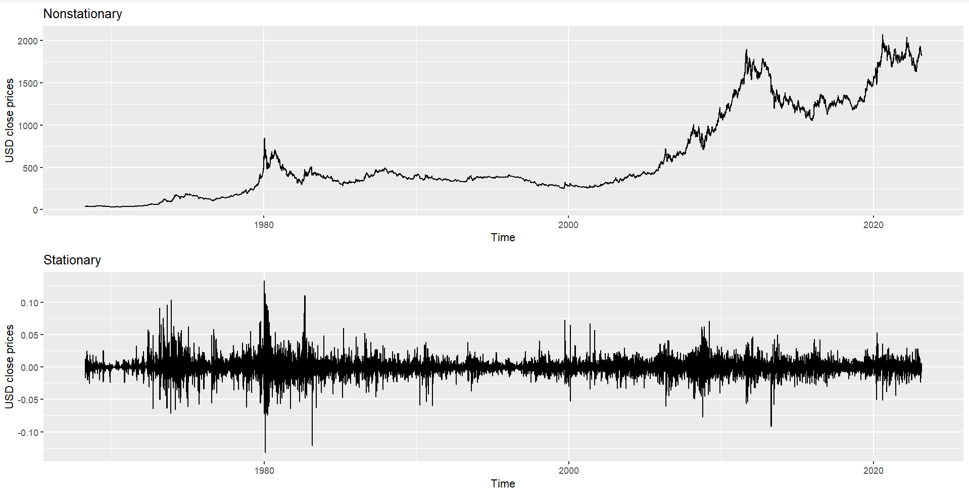
Let's plot it!
It can be visually visible in plot_Stat that the movement is never far from zero, which indicates that the daily return has smaller and constant variance, constant mean, and no trend at all.
Therefore, plot_Stat is the example of stationary movement.
# ##------------Plot--------------------------------------------------------------------------------------------------------------------------------

# First visualization
plot_NonStat <- df_DataEngineered %>%
ggplot(aes(x=date,y=close))+
geom_line()+
labs(x="Time",y="USD close prices")+
ggtitle("Nonstationary")

plot_Stat <- df_DataEngineered%>%
ggplot(aes(x=date,y=dr))+
geom_line()+
labs(x="Time",y="USD close prices")+
ggtitle("Stationary")

##Visualize both in one Plot
grid.arrange(plot_NonStat,plot_Stat)